
01
Design goalStart with the sensing question
The study begins with an intuitive engineering question: how far does 850 nm light travel through layered tissue, and where could a wearable detector recover a useful signal?
Explore tissue optics, photonics, spectral rendering, lenses, filters, cameras, and detector pipelines with open scientific engines—then inspect the fields, assumptions, and design tradeoffs.
Tissue light transport
Spectral optical systems
Sensor and camera pipelines
Example study
This real workflow starts with an everyday idea—a near-infrared wearable sensor—and progressively turns it into a bounded physical model, a GPU computation, visual evidence, and a defensible next experiment.
1,000,000
Bounded GPU Monte Carlo transport
850 nm
A common wearable-sensing wavelength
0.5 mm
60 × 60 × 40 tissue grid
RTX 4090
MCX through pmcx 0.7.1
01
Design goalThe study begins with an intuitive engineering question: how far does 850 nm light travel through layered tissue, and where could a wearable detector recover a useful signal?
02
Physical modelVicena converts layer thicknesses, absorption, scattering, anisotropy, refractive index, source position, and voxel size into an explicit MCX configuration.
03
GPU computeOne million photon histories move through the voxel volume with Fresnel boundaries. The managed job keeps the engine version, seed, grid, and optical assumptions attached.
04
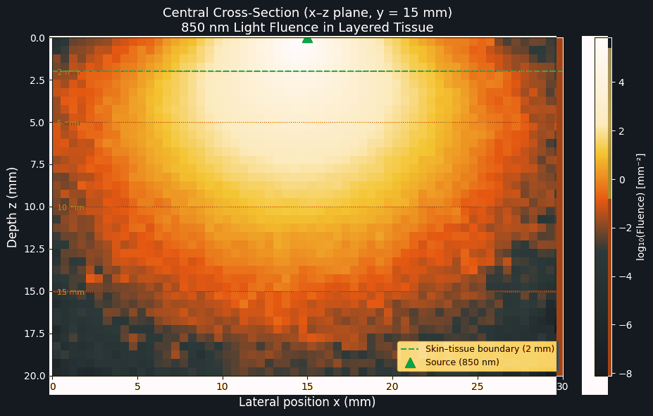
Visual evidenceThe three-dimensional fluence field becomes centre-plane heatmaps, depth attenuation, target-depth summaries, and lateral-spread profiles instead of one opaque scalar.
05
Quality gatePenetration, absorbed fraction, boundary behavior, photon-count sensitivity, voxel sensitivity, and detector assumptions are separated from experimental validation.
06
Next designSource–detector spacing, wavelength, tissue layers, optical properties, and photon budget can be changed while preserving the same reproducible workflow contract.
Real workflow artifacts
Every figure below comes from the executed MCX notebook. The three-dimensional result remains available behind the plots, so the agent can answer follow-up questions without rebuilding the science from a screenshot.
The real MCX result shows the rapid change in fluence across a 30 × 30 × 20 mm tissue volume. The source, skin boundary, and depth markers remain connected to the executed configuration.
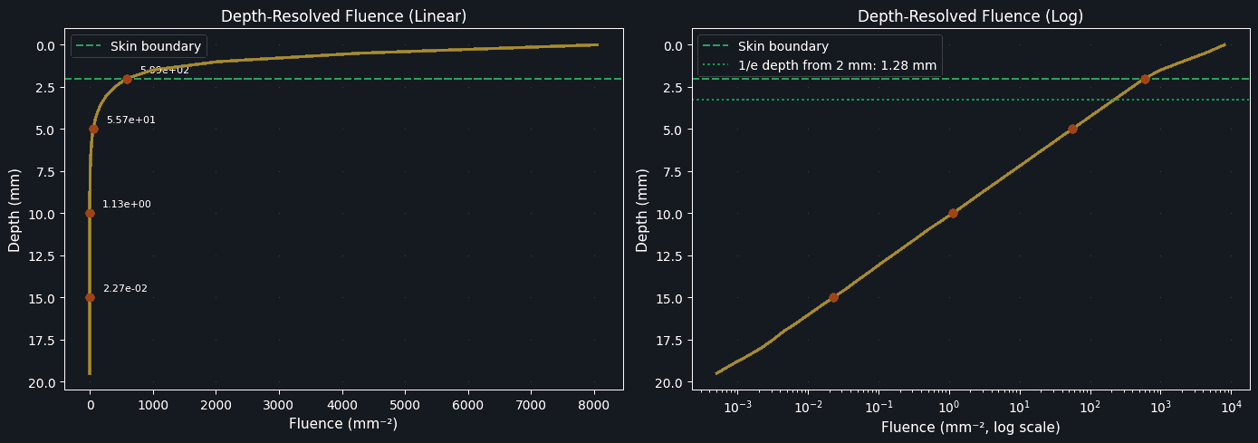
Linear and logarithmic views expose both the near-surface maximum and the orders-of-magnitude falloff that matters for detector placement.
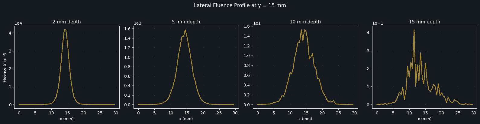
Profiles at 2, 5, 10, and 15 mm show how scattering broadens the illuminated region while the available fluence decreases.
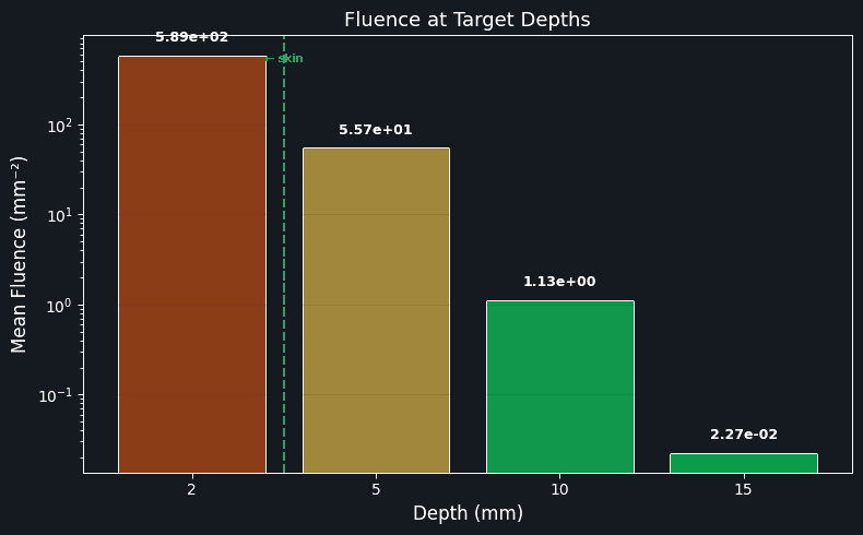
The result can be reduced into an engineering comparison without losing the underlying three-dimensional array and notebook.
Scientific packages

pmcx 0.7.1
GPU photon transport
Traces photon histories through voxelized media for tissue optics, fluence, absorption, and detector-placement studies.
Official project
1.34
FDTD electromagnetics
Solves time-domain Maxwell equations for photonic structures, transmission, resonances, fields, and device response.
Official project Photonic band structures
Computes electromagnetic modes and dispersion relations for periodic dielectric structures and photonic crystals.
Official project
3.9
Spectral rendering
Models light transport through surfaces, materials, lenses, filters, cameras, and differentiable imaging systems.
Official project
0.6.2
Multi-objective optimization
Explores optical design tradeoffs such as signal, absorption, geometry, robustness, and competing objectives.
Official project
1.5.2
Sensitivity analysis
Quantifies how uncertain optical properties and design variables influence simulated outputs and decisions.
Official projectScientific capabilities
Vicena routes the question to the appropriate open scientific engine and keeps model boundaries explicit—from scattering tissue to spectral surfaces and sensor pipelines.
Model absorption, scattering, anisotropy, refractive-index boundaries, sources, and voxelized media with GPU MCX.
Use registered Mitsuba workflows for surface, lens, filter, spectral-rendering, and differentiable-imaging studies.
Connect simulated light to filters, quantum efficiency, image formation, calibration, noise, demosaicing, and downstream analysis.
Compare wavelengths, geometries, optical properties, source–detector spacing, robustness, and multi-objective tradeoffs.
Evidence discipline
The value is not a colorful heatmap by itself. It is the connection between the question, physical assumptions, managed execution, arrays, plots, provenance, and the next design decision.
Scientific boundary
Start with your design
Start with a real optical design question. Vicena can select the workflow, prepare the model, run bounded compute, and return the visual evidence.